

So far in this article series, we have discussed the role of the Finance Commission (FC), the methodology used by the 15th FC that has sparked controversy, and the socio-economic concerns and demands of the five southern states.
In this article, we will examine expert perspectives on some of the major issues raised by the southern states, assessing how justified their concerns are and exploring the different approaches proposed to address these challenges. The expert perspectives will include those of renowned economists and public finance specialists, along with additional analytical insights. At the same time, we will present diverse viewpoints to ensure a balanced and comprehensive understanding of the debate.
1. Debate on Fiscal Transfers and Regional Equity
Pinaki Chakraborty, Former Director and Professor at the National Institute of Public Finance and Policy (NIPFP) and Economic Advisor to the 14th FC, has addressed the ongoing debate around fiscal transfers and regional equity. He responds to the grievance raised by southern states that, despite contributing a higher share of taxes to the central pool, they do not receive a proportionate share in tax devolution. These states argue that their revenues are being diverted to poorer states, such as Uttar Pradesh and Bihar.
Southern states’ grievances arise from the income distance formula. Income distance, the highest-weighted indicator in the distribution formula, is calculated as the difference between a state’s per capita GSDP and the per capita GSDP of the highest-income state. Simply put, the poorer the state, the more funds it receives.
Income Distance Formula by the Finance Commission
a. Three-Year Average Per Capita GSDP (GSDPPCᵢ): Three-year (2016-17 to 2018-19) average of per capita GSDP of iᵗʰ State (GSDPPCᵢ)
b. Income Distance (dᵢ): dᵢ is the distance (difference) of iᵗʰ state’s GSDPPCᵢ from the third-highest state’s, namely Haryana’s, GSDPPC
c. Income Distance (Dᵢ): Dᵢ = dᵢ * POPᵢ₂₀₁₁
Chakraborty contends that this grievance overlooks the interdependent nature of income generation in India’s integrated economic market. For example, a company may be headquartered in one state and pay taxes there, while generating a significant portion of its revenue through sales, consumption, and operations in other states. In such cases, tax collection data does not accurately represent where economic activity is taking place. He argues that using tax collection and contribution as the primary basis for resource devolution would be regressive. It would disproportionately benefit high-income states while undermining the principle of redistributive justice, a fundamental tenet of India’s federal fiscal framework.
He highlights that labour migration from poorer northern states has significantly contributed to the economic prosperity of the southern states. Migrant workers have kept labour costs low, enabling higher value addition and output in the destination states.
Responding to the complaints of some states about not receiving adequate financial assistance from the Centre, he explained that when tax devolution is insufficient to cover a state’s pre-devolution revenue deficit, the FC provides post-devolution revenue deficit grants to bridge the gap. These grants are grants to cover the shortfall in revenue expenditure after assessing the post-devolution deficit based on projected fiscal capacities and needs. They are untied and fixed in absolute terms, meaning the amount does not change based on any factors and is not linked or relative to any changing indicator, thereby ensuring a stable and predictable flow of resources to the states. For instance, Kerala received the largest share of revenue deficit grants for the period 2021–26 under the 15th FC, out of all 26 recipient states. Similarly, Andhra Pradesh, which saw a decline in its share of tax devolution following its bifurcation, was awarded such grants to help maintain fiscal stability. Therefore, any meaningful assessment of inter-state fiscal equity must take into account both tax devolution and revenue deficit grants to fully understand the total financial support provided through the FC.
Rathin Roy, Former Director of NIPFP and Economic Advisor to the 13th FC, supports this line of reasoning. He reiterates that a company does not generate all its income in the state where it is headquartered and pays taxes. Instead, value is created through consumption and economic activity spread across the country.
On the same issue, D. Subbarao, former Governor of the Reserve Bank of India, and Arvind Subramanian, former Chief Economic Adviser, stated that cross-subsidisation, referring to the transfer of resources from richer states to poorer states through central tax devolution, is both necessary and desirable, at least to a certain extent. Subbarao noted that such fiscal transfers are a common feature of most federal systems worldwide. He emphasised that it is incumbent upon the richest states to cross-subsidise the poorest. However, he also cautioned that there must be limits to such cross-subsidisation, and he senses that India may be approaching those limits.
Subramanian, while discussing the redistribution of resources, argues that redistribution should be understood as a core feature of nation-building and not merely as a response to fiscal imbalance. He maintains that one must go beyond the usual narrative of richer states transferring more to poorer states and consider other often-overlooked dimensions. For example, Bihar could argue to Tamil Nadu: “We provide you with cheap labour. Therefore, while you may be transferring fiscal resources, we are transferring human resources.”
Historical context deepens the understanding of regional disparities. Devesh Kapur, a Professor of South Asia Studies at Johns Hopkins University, highlights that regional imbalances are not new. He refers to the Freight Equalisation Policy, introduced in 1952 and in force until 1993, which effectively penalised mineral-rich eastern states such as Bengal, undivided Bihar, and Orissa. Under this policy, the central government subsidised the cost of transporting key industrial raw materials such as coal, iron ore, steel so that factories across the country could receive inputs at uniform prices. While designed to promote balanced industrialisation, it had the opposite effect: heavy and medium industries grew outside the mineral-rich eastern region, leading to long-term industrial stagnation in states that should have naturally benefited from their resource base.
To make the distribution of resources fairer and provide stronger incentives for states to improve their per-capita GSDP, S. Raja Sethu Durai, Professor of Economics at the University of Hyderabad and BITS Pilani, suggests a small modification to the income-distance formula.
First, the per-capita GSDP values used by the previous Finance Commission are taken as the base. Next, the average per-capita GSDP of all states for the most recent three years is calculated. The growth rate between these two averages represents the minimum expected increase in per-capita GSDP for every state. Using this expected growth rate, an “expected per-capita GSDP” is computed for each state. Income distance is then measured as the gap between a state’s expected per-capita GSDP and that of the highest-income state. This gap, multiplied by the state’s population, determines its share in the distribution formula. These expected values can serve as the new base for income-distance calculations in future Finance Commissions.
Deriving income distance from this expected level solves two key problems. First, it does not penalise states that grow faster than expected; instead, it places the burden on states that grow below the expected level by making them account for the gap they fail to cover. Second, since this expected level becomes the base for the next Commission’s calculations, it encourages better-performing states to maintain their growth momentum while pushing slower states to grow faster to catch up.
While concerns raised by southern states have largely shaped the public discourse on fiscal transfers, a broader look reveals that the issue is not exclusively a “South vs North” divide. A more accurate framing of the problem, as presented by Mint, is that of a “rich versus poor” imbalance. Their analysis highlights that states contributing more to the central exchequer are not confined to the South alone; Western states such as Maharashtra and Gujarat, as well as northern states like Punjab and Haryana, also contribute significantly more than they receive. For instance, Karnataka reports that for every tax rupee it contributes, it receives only 15 paise in return. Kerala receives 25 paise, while Tamil Nadu receives 29 paise. In contrast, the redistribution heavily favours some northern states: Uttar Pradesh receives ₹2.73 for every ₹1 contributed, and Bihar receives an even higher ₹7.06

However, when tax devolution is viewed on a per capita basis, states like Bihar and Uttar Pradesh actually receive less than southern states such as Kerala and Karnataka. This indicates that India’s fiscal transfers are less progressive than commonly assumed. International comparisons reinforce this point: while the poorest one-fourth of states in India receive about 22% of total transfers from the Centre, the poorest quartile in South Africa receives roughly 30%, and in Brazil nearly 36%.
The Mint analysis challenges the simplistic binary of North vs South and underscores the need to understand the issue beyond regional lines. It also draws attention to intra-state inequalities, for example, regions like Western Uttar Pradesh are more prosperous than some parts of southern India, making the debate on regional equity more nuanced.
2. Population Data: Shift from 1971 to 2011
The shift to using 2011 population figures became the primary source of criticism from southern states, who argued that this approach unfairly penalised them for successfully controlling population growth. They therefore demanded that the 1971 Census continue to be used as the basis for distribution. The Union government and the 15th FC have defended the use of 2011 Census data, arguing that the 1971 population figures no longer reflect current demographic realities. Over the decades, states have experienced diverging trends in fertility, age structure, and migration, factors that the 2011 data captures more accurately. The Commission noted that its terms of reference required the use of 2011 data to ensure fiscal equalisation.
Historically, the population held a dominant weightage in the FC’s devolution formula. In the Early FCs, population accounted for about 80–90% of the distribution of personal income tax and Union excise duties. This emphasis continued up to the 7th FC. However, from the 9th FC onward, the weightage declined significantly to 10%, and in recent Commissions, it has fluctuated between 15% and 25%.
Lekha Chakraborty, an economist and professor at the NIPFP, argued that giving excessive weightage to the 2011 population data is an injustice to the states that have successfully controlled their population growth. Due to the reduction in transfers from the Centre, largely due to slower population growth, these states are finding it harder to manage their budgets. She points out that, as a consequence, they may be forced to cut costs, such as delaying or reducing government employee salaries and pensions, and scaling back spending on welfare schemes, leading to a situation of fiscal austerity, where governments must impose strict spending controls due to a shortage of funds.
On the other hand, Pranay Kothaste, Deputy Director at Takshashila Institution, argues that general-purpose transfers (like FC transfers) are not meant to favour some states or punish others. Instead, their goal is to make sure that every state has enough financial resources to provide similar quality public services such as health, education, and infrastructure, without having to impose higher taxes on its citizens. From this perspective, it is reasonable to use the most recent population data. According to him, using outdated data such as the 1971 Census effectively turns fiscal transfers into tools for incentivising family planning, something they are not intended to do. He argues that population control should be addressed through targeted expenditure programs, not by distorting tax devolution formulas.
Furthermore, he contends that denying funds to individuals in poorer regions simply because their areas remain underdeveloped goes against the spirit of the Indian Republic. If one accepts the logic of a “southern versus northern” divide in tax transfers, it would also imply opposition to intra-state transfers—for example, from Bengaluru to Bidar, or from Whitefield to underdeveloped parts of south Bengaluru.
M Govinda Rao, a Member of the 14th FC and Former Director NIPFP, also endorsed the use of updated demographic data in resource distribution. He emphasised that public services must be provided to the entire population, and therefore, the latest population data should be used when making such estimates.
Adding to the debate, Rathin Roy pointed out that the shift to 2011 population figures should not be viewed in isolation. He argued that the impact of this change depends not only on the base (i.e., the population data used) but also on the weight assigned to it in the formula. For example, if the population had been given a 25% weight, it would have exerted a stronger influence on the devolution formula. But when the weight is reduced to 10% or 15%, even a state with a smaller 2011 population is not significantly disadvantaged. In that sense, he suggests that concerns about southern states losing out may be overstated, especially if demographic achievements are also recognised, as the terms of reference encourage.
3. Demographic Performance and Tax Effort Parameters
As a way to balance the use of 2011 population data and acknowledge the efforts of states that successfully controlled population growth, the 15th FC introduced a new parameter: demographic performance, aimed at rewarding states for achieving lower fertility rates.
Demographic Performance Formula by Finance Commission
a. Age-Specific Fertility Rate (ASFR): ASFRi,k = (Number of live births in the last year to females in the kᵗʰ age group in the iᵗʰ state) / (Mid-year female population in the kᵗʰ age group in the iᵗʰ state)
Note: The female population recorded in the Census 2011 for each age group is taken as the mid-year female population.
b. Total Fertility Rate (TFR) of the iᵗʰ State: TFRᵢ = 5 × Σ ASFRi,k
Where k = 15–19, 20–24, 25–29, 30–34, 35–39, 40–44, 45–49.
c. Demographic Performance (DP): DPᵢ = (1 / TFRᵢ) × POPᵢ,₁₉₇₁
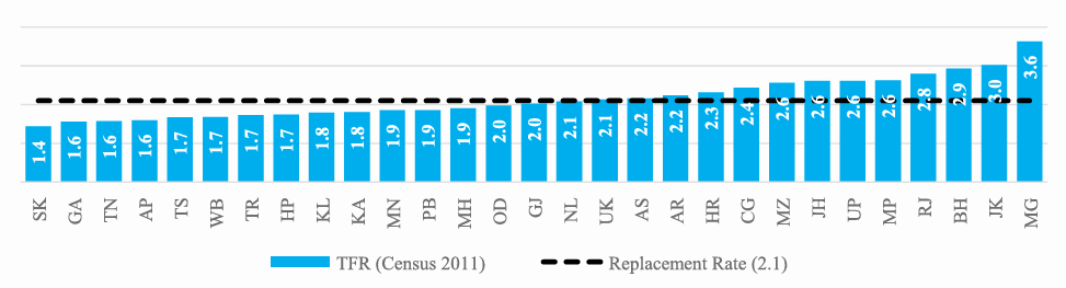
While this was welcomed in principle, it has faced criticism over the way it was calculated. Instead of simply using the inverse of the Total Fertility Rate (TFR) for each state, the Commission multiplied the inverse TFR by the state’s 1971 population.
This approach resulted in some unexpected outcomes. According to a study by the Accountability Initiative at the Centre for Policy Research, states such as Uttar Pradesh and Bihar ranked higher due to their large population base in 1971, despite having higher fertility rates. In contrast, states such as Telangana and Himachal Pradesh, which have successfully maintained low TFRs, did not gain as much because of their smaller 1971 population shares.
Rajeev Gowda, Vice-Chairman of the State Institute for Transformation of Karnataka, had also expressed scepticism about the extent to which the demographic performance parameter could offset the impact of using population as a criterion. He maintained that incorporating the population parameter would inevitably reduce the share of southern states, a concern that has ultimately materialised.
Nilakantan R.S., data scientist and author of South vs North: India’s Great Divide, highlights how population dynamics can lead to fiscal imbalance across India’s regions. He notes that regional financial disparities are common worldwide, but in many federal systems, they are corrected through tax redistribution policies. For instance, in the United States, the traditionally poorer southern states receive greater financial support from the federal government as compared to the wealthier industrial North. Similarly, in Germany, although the western region remains significantly more prosperous than the former Communist East, federal mechanisms help narrow this economic gap. Comparable fiscal arrangements exist in countries as diverse as Spain, China, and the United Kingdom.
However, Nilakantan argues that India’s situation is unique in two major ways. First, the development and economic resource gap between India’s regions, particularly between the North and the South, is far more pronounced than in other countries. Second, and more importantly, the demographic trend in India is the opposite of what is seen elsewhere. In most federal nations, the richer regions tend to be the more populous ones, due to higher levels of urbanisation and migration, which enables them to contribute more to the national economy. In India, on the other hand, the poorer states have larger and faster-growing populations, driven primarily by high TFRs rather than migration.
As a result, this redistribution model becomes more challenging, especially when southern states are themselves dealing with their own socio-economic issues, yet are still expected to financially support regions that remain more populous and underdeveloped.
Another demographic concern raised by southern states is the rapid growth of their elderly population. States such as Kerala, Tamil Nadu and Andhra Pradesh have significantly lower fertility rates, and with life expectancy increasing, a larger share of their population is now elderly. This creates higher fiscal demands for healthcare, pensions and social welfare, which they argue must be reflected in the tax devolution formula. Yadawendra Singh and Lekha Chakraborty, in one of their papers, analyse this issue by incorporating the elderly population, measured as a percentage of the working-age population, into the FC criteria. Their study tests multiple scenarios, starting with adding a small weight for the elderly to the existing formula, and then assigning a much higher weight by reducing or removing the weightage given to the total population and tax effort. Across all versions, the results consistently show that ageing states, especially Kerala, followed by Tamil Nadu and other southern and western states, gain a larger share of resources, while highly populous northern states lose a part of their current allocation.
A similar debate surrounds the tax-effort criterion. Critics argue that multiplying tax effort by the 1971 population distorts its meaning. It raises the question of how a state’s historical population can reflect its present efficiency in tax collection. For example, Uttar Pradesh scores higher than Tamil Nadu on tax effort, despite the latter showcasing better fiscal performance.
Tax Effort Formula by Finance Commission:
a. Average Per Capita Own Tax Revenue (Tᵢ): Tᵢ = Three-year average (2016–17 to 2018–19) of per capita own tax revenue of the iᵗʰ State
b. Average Per Capita GSDP (𝐺SDDP𝐶ᵢ̄): 𝐺SDDP𝐶ᵢ̄ = Three-year average (2016–17 to 2018–19) of per capita GSDP of the iᵗʰ State
c. Tax Ratio (tᵢ): tᵢ = Tᵢ / 𝐺SDDP𝐶ᵢ̄
d. Tax Effort (TEᵢ): TEᵢ = tᵢ × POPᵢ,₁₉₇₁
The FC’s reasoning behind scaling population data with factors such as income distance, tax effort, and demographic performance makes the formula more progressive and enables states to undertake necessary expenditure for providing services to their residents.
4. Rising Share of Cesses and Surcharges
Another major concern raised by states is the increasing share of cesses and surcharges in the government’s gross tax revenue, as these collections are not part of the divisible pool. The states argue that the Centre’s overreliance on cesses and surcharges is reducing the shareable portion of its gross tax revenue.
The share of cesses and surcharges rose from 8.16% of gross tax revenue in 2011–12 to 28.1% in 2021–22, though it came down to 14.5% in 2023–24 due to reduced duties on petrol and diesel.
Until 2023–24, the Centre levied at least 13 cesses and 4 surcharges. These cesses were applied in sectors such as agriculture (Agriculture Infrastructure and Development Cess), health and education (Health and Education Cess), and infrastructure (Road and Infrastructure Cess), among others.
From 2024–25 onwards, the government rationalised these, reducing the number of cesses to 7, though the number of surcharges remained at 4. Even after the introduction of GST, which subsumed many cesses, the government continued to impose new ones like the Swachh Bharat Cess and Krishi Kalyan Cess.
Despite this rationalisation, total collections from cesses and surcharges have steadily increased. The Centre’s collections rose from a little over ₹1 lakh crore in 2014–15 to ₹2.17 lakh crore in 2019–20, and then grew to ₹5.4 lakh crore in 2024–25. They are expected to reach ₹5.91 lakh crore in 2025–26.
D.K. Srivastava, Chief Policy Adviser at EY India and a Member of the Advisory Council to the 15th FC, pointed out that the fiscal imbalance has worsened after GST. Since states cannot independently change GST rates, their ability to raise revenue has become limited. Meanwhile, since the Centre’s tax collections are not growing fast enough, it has increasingly relied on cesses and surcharges to fund its spending, as these revenues do not have to be shared with the states.
Earlier FCs had recommended that the Union Government review the current position with respect to the non-divisible pool arising out of cess and surcharges and take measures to reduce their share in the gross tax revenue. More recently, the 14th FC had also flagged the growing share of cesses and surcharges as problematic.
Moreover, the Comptroller and Auditor General (CAG) pointed out the lack of transparency in the Union’s reporting of cess utilisation. Of the ₹2.74 lakh crore received through around 35 cesses and levies in 2018–19, only ₹1.64 lakh crore (about 60%) was transferred to the respective Reserve Funds and Boards, while the rest remained in the Consolidated Fund of India.
Data presented by Finance Minister Nirmala Sitharaman in the Lok Sabha shows that ₹5.7 lakh crore collected via cesses and surcharges since 2019–20 is projected to remain unspent by March 2026. Cess utilisation has also stagnated in recent years, peaking at ₹3.36 lakh crore in 2021–22, then falling to ₹2.57 lakh crore in 2023–24, with only modest increases expected in 2024–25 and 2025–26.
The 15th FC commissioned a study on this issue by the Vidhi Centre for Legal Policy. The report raised concerns over the prolonged use and misuse of certain cesses. It is recommended that long-standing cesses or those with evidence of non-utilisation or diversion should be abolished. The report also advised that cesses be limited to narrowly defined purposes, include revenue estimates, and be governed by laws with sunset clauses to ensure they do not continue indefinitely. It further argued that surcharges should not substitute for progressive taxation, suggesting that income tax rates themselves be rationalised to reflect progressivity more transparently.
5. GST Compensation Cess:
Another argument presented by the southern states concerns their limited tax-raising capacity and the discontinuation of the GST compensation cess, along with their demand for its renewal. When GST was introduced, states relinquished their independent taxation powers, and the authority to tax goods shifted from the state of origin to the state of destination. To offset this loss, the Centre had promised to ensure a 14% annual growth in states’ GST revenue for five years (2017–2022), calculated over the 2015–16 base year. This guarantee was funded through the compensation cess levied at varying rates on luxury, sin, and demerit goods such as cigarettes, pan masala, gutkha, other tobacco products, soft drinks, and certain categories of automobiles.
Although the cess was originally expected to be phased out in 2022, the COVID-19 pandemic severely affected collections, forcing the Centre to borrow ₹2.69 lakh crore to fulfil its compensation commitments to the states. The government later extended the levy and collection of the compensation cess until March 2026, but only for the repayment of these loans, while GST compensation to states ended after June 2022. With the loans now nearly settled, the government anticipates a surplus of around ₹40,000 crore from the cess, which states argue should be shared with them.
Many states, particularly those running large fiscal deficits and carrying significant debt, fear that recently announced reductions in GST rates or cuts in certain slabs will negatively affect their revenues. Given their heavy dependence on GST as a stable revenue source, they are demanding a renewed compensation mechanism. Specifically, they are pressing for a minimum five-year compensation guarantee using 2024–25 as the base year, with protection of at least 14% annual revenue growth, similar to the terms provided during the first five years of GST.
Pratik Jain, Partner at PricewaterhouseCoopers India, while speaking on the potential tax losses, noted that it is difficult for the Centre to keep compensating States for routine tax losses. While additional funds can be allocated for areas like infrastructure, States must strengthen their own tax systems by plugging leakages, widening the tax base, and attracting investment to become self-sufficient. In a country like ours, regular compensation to States for tax shortfalls is not a sustainable option for the Centre.
The government’s recent decision to integrate the compensation cess into the GST rate structure will help boost States’ revenue receipts. The Lok Sabha passed the Central Excise (Amendment) Bill to levy excise duty, replacing the cess, on tobacco and related products. As a result, the revenue collected will now be part of the divisible pool, of which 41% will be shared with the States. Additionally, luxury automobiles and aerated drinks, which earlier attracted a 22% cess in addition to 28% GST, now fall under the 40% GST slab with no additional cess. The increase in the slab will also lead to higher revenue for the States.
The debate surrounding the Finance Commission’s devolution formula is far more nuanced than the common narrative of a “southern versus northern” divide. Expert perspectives suggest that the real fault line is shaped by historical developments, demographic trends, and uneven economic capacities. While the Commission aims to balance equity and efficiency, experts have raised concerns about aspects such as the use of population multipliers and the rising share and underutilisation of cesses and surcharges. Southern states argue that, since they contribute more to the national tax pool, they should receive a larger share of devolution. However, this claim is countered by considerations of the spatially interdependent nature of income generation, the role of migration, and the inclusion of revenue deficit grants in overall fiscal distribution. As India prepares for the next Finance Commission, the challenge will be to strike a careful balance between equity and efficiency – supporting lagging states without penalising those that have progressed, while designing a formula that strengthens the Union and empowers its diverse states.
Table: Summary of Key Issues and Expert Perspectives on Finance Commission Debates
Topic | Issue Raised | Expert Comments / Perspectives |
1. Fiscal Transfers & Regional Equity | Southern states argue they contribute more to the central tax pool but receive less in return, subsidising poorer northern states. | • Pinaki Chakraborty: Tax collection does not reflect where value is created; redistribution is essential for equity. Migrant labour from poorer states supports southern growth. Revenue deficit grants must be included in assessing fairness. |
2. Population Data Shift: 1971 → 2011 | Southern states feel penalised for controlling population growth and demand the continued use of 1971 data. | • Government & 15th FC: 2011 data reflects current demographic needs; required for equalisation. |
3. Demographic Performance & Tax Effort | Criticism that linking both parameters to the 1971 population favours large, high-fertility states like UP/Bihar and limits southern gains. | • Accountability Initiative: 1971 multipliers distort rankings—high-fertility states score better than low-fertility ones. |
4. Rising Cesses & Surcharges | States claim increasing cesses reduce the divisible pool; utilisation lacks transparency. | • D.K. Srivastava: States have limited tax flexibility post-GST → Centre relies more on cesses. |
5.GST Compensation Cess | Southern states argue limited tax-raising capacity and GST cess discontinuation reduce revenue stability; demand renewal | • States want a new 5-year compensation guarantee, using 2024–25 as base year with 14% growth. • Pratik Jain (PwC): Continuous compensation is unsustainable; states must widen tax base, reduce leakages, attract investment. • Recent reform: Compensation cess integrated into GST rates; revenue enters divisible pool (41% to states); luxury cars & aerated drinks now in 40% slab, boosting state revenues. |
Until now, we have focused mainly on the theoretical aspects of the debate and have not examined the quantitative dimension. In the next article of the series, we will analyse the issues discussed in the previous blogs using data-backed evidence, mapping trends, and verifying the claims made by the southern states, with the aim of providing a more nuanced and objective view.